Introduction
In this blog post, we are going to analyze the keys and tags from OpenStreetMap (OSM) with a particular interest on environmental and agricultural topics.
To follow along, here is the codebase associated with this blog post: https://github.com/NoeFlandre/osm-stats
Overview
The first step to perform such an analysis is to download the dataset of statistics including all keys and tags from OSM data which is available at the following link: https://taginfo.openstreetmap.org/download/taginfo-db.db.bz2
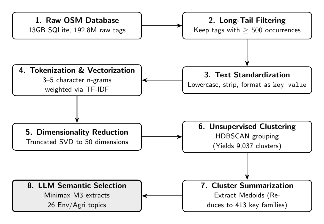
Once extracted, the reader will find a file of roughly 13GB with an SQLite database.
First global stats
To get started we need to understand what is a key and what is a tag. A key is typically a single word which describes a category of OSM polygon. For instance “building” is a key. A tag, is simply a pair of (key, value). An example of a tag would be (building, house). So a polygon of a house on OSM will belong to the key “building” and most likely have a tag “building=house” which corresponds to the (key, value) = (building, house).
Now let’s have a look at some descriptive stats from our database:
- The total number of distinct keys is 110,706.
- Likewise, the total number of tags is 192,821,586.
- The total number of occurrences is 3,892,388,715.
We can already conclude that this is a fairly large database.
Most popular keys and tags
If we want to take a first glance at the data, we can check what are the top 10 keys and top 10 tags (key=value pairs).
For the keys, we can see that basic infrastructure dominates:
- building (~699.6 million entries)
- source (~310.2 million)
- highway (~296.3 million)
- addr:housenumber (~180.9 million)
- addr:street (~170.0 million)
- addr:city (~131.3 million)
- addr:postcode (~115.2 million)
- name (~114.1 million)
- natural (~92.2 million)
- surface (~78.7 million)
The tags are confirming this first observation:
- building=yes (~556.4 million)
- highway=residential (~69.4 million)
- building=house (~66.1 million)
- highway=service (~64.6 million)
- surface=asphalt (~36.2 million)
- source=microsoft/BuildingFootprints (~35.8 million)
- natural=tree (~33.6 million)
- highway=footway (~31.6 million)
- highway=track (~29.6 million)
- waterway=stream (~29.0 million)
Should we just remove some obvious keys?
What we would like is to cut through the noise and only keep the keys and tags we are interested in (anything relevant to topics like agriculture, environment and so on). One could have the idea to directly remove the “building” key completely but before doing that, let’s have a look at the first 20 tags with “building” as a key:
| value | count_all |
|---|---|
| yes | 556,451,624 |
| house | 66,181,816 |
| residential | 16,123,805 |
| detached | 10,056,176 |
| garage | 8,122,742 |
| apartments | 7,784,487 |
| shed | 4,495,922 |
| industrial | 2,608,502 |
| roof | 2,450,761 |
| hut | 2,447,641 |
| farm_auxiliary | 2,366,983 |
| semidetached_house | 1,974,860 |
| terrace | 1,478,303 |
| commercial | 1,455,301 |
| school | 1,345,309 |
| retail | 1,274,921 |
| construction | 1,132,478 |
| outbuilding | 1,084,337 |
| garages | 1,054,157 |
| greenhouse | 821,293 |
| barn | 805,630 |
| cabin | 657,564 |
| static_caravan | 557,489 |
| service | 548,879 |
| warehouse | 473,553 |
| bungalow | 440,894 |
| church | 433,987 |
| farm | 414,913 |
| allotment_house | 349,247 |
| carport | 338,130 |
| office | 304,623 |
| ruins | 290,506 |
| public | 213,143 |
| civic | 212,355 |
| university | 176,658 |
| hospital | 170,684 |
| hotel | 160,423 |
| kindergarten | 127,484 |
| chapel | 119,655 |
| boathouse | 118,131 |
| ger | 107,876 |
| mosque | 107,555 |
| storage_tank | 105,426 |
| manufacture | 99,828 |
| hangar | 95,179 |
| bunker | 74,512 |
| dormitory | 73,721 |
| silo | 65,809 |
| train_station | 60,106 |
| college | 55,587 |
As we can see the tags are including many elements we are not interested in (e.g bunker, college and so on). However some tags could be of interest from an environmental / agriculture perspective (e.g greenhouse, farm). So simply discarding all occurrences with a “building” key is not the right solution. On top of that, we saw earlier that the entire set is including 110,706 keys and going through each of them would take a while… We therefore can’t offered to do a fine filtering manually.
Filtering at scale
One of the critical issue with OSM data is that the tags are not standardized, in other words it seems like each contributor is fairly free to annotate a polygon using free form text. Moreover we can assume that some typos might exist in the tags. Therefore it is likely that among the 192,821,586 tags, we may have a very long tail of tags which are not used that often since they come from a specific user notation.
Removing tags with low occurrences
In order to first clean up this database and only keep prominent tags, we can decide to only keep tags such that count_all >= 500. This simple filtering brings down the number of unique (key, value) pairs from 192.8 M to 224,123. By doing this filtering, the total number of occurrences goes from 3,892,388,715 to 3,350,015,993, so the long tail filtering dropped roughly 14% of occurrences in total while dramatically cleaning up the number of tags (roughly compressing the number of tags by a factor or 860). In simpler terms, we significantly reduced the complexity of our codebase while preserving a satisfactory number of samples.
Standardizing tags
Since OSM tags could be messy (for example we could think of tags having “Landuse” and “landuse”), we want to turn them into clean pairs. To do so we convert each string into lowercase, we strip to remove any unwanted space, we handle missing values by mapping them to “none” and finally we joint keys and values using the pipe “|” as a joiner since it never appears in our OSM values. Every tag now looks clean and resemble something like this : “landuse|farmland”.
Tokenizing our strings
Now that we have clean tags, we can try to cluster them, in order to gather together tags which belong to a similar topic. To do so we need to turn our strings into vectors. We have two options for that: either tokenize them at the word-level or at the character-level. Tokenizing at the word level would require exact matches, which is a harsh condition and also can be too strict. Suppose the context where a user would have made a type and wrote “lanuse|farmland” instead of “landuse|farmland”. Tokenizing at the word level would consider “landuse” and “lanuse” as two different words while they are the same. That’s why tokenizing at the character level might be a better pick here. A good solution here is to use n-grams (i.e a sliding window of N characters through the word). For instance the 3-grams from the word “landuse” are “lan”, “and”, “ndu”, “dus” and “use”. This way, even when we have a typo, two words still share a high similarity. For example “landuse” and “lanuse” share the 3-grams “lan” and “use”. A good tradeoff as well is to choose a range of n-grams from 3 to 5 grams (2 being too noisy since 2-grams are shared across two many words, and 6+ being too specific).
Turning tokens to vectors
On top of this tokenization, we are going to need a way to analyze these n-grams. If we were to simply count n-grams, this would treat each n-gram as equally important. However this is not a good approach since some n-grams are very common in English like “ing” and therefore non informative, while some n-grams are rather rare like “g|y” (the boundary between “building” and “yes”) and in this case, is very informative. In order to tackle this issue, we can use TF-IDF which stands for Term Frequency - Inverse Document Frequency. The idea is to weight each n-gram by how rare it is across the whole dataset. The term frequency is the count of the n-gram in the current string while the inverse document frequency down-weights n-grams that appear in many strings and up-weights n-grams appearing only in a few. The intuition behind using this is exactly what we described before: a rare n-gram is informative while a common one is not.
As an implementation detail, we decide to drop any n-gram that appears only in one tag string since it carries no clustering signal. This is just an optimization to keep a vocabulary that actually connect tags together. The output of this transformation is a sparse matrix of shape (224,123; 396,969) each row is a tag string while each column is surviving n-gram. The cell at position (i, j) carries the weight of the TF-IDF for the n-gram j of the tag string i. In this matrix we have a sparse density of 0.014% which means that each string only activates a ver small handful of the 396,969 possible n-grams. At this stage, we have effectively turned each tag into a vector of dimension 396,969. In this space, two tags sharing many n-grams end up close to each other while those sharing none are orthogonal.
Dimensionality reduction
The clustering algorithm we are going to use later is HDBSCAN, which computes pairwise distances between every pair of points. For a full pairwise matrix this is O(n^2* d) where n is the number of points and d the number of dimensions. In our case we have d = 396,969 and n = 224,123 which is intractable. However we are dealing with a sparse matrix, which makes it possible to rather compress it into a dense matrix. To do so we are using Truncated Singular Value Decomposition, which is a dimensionality reduction technique which approximates a matrix by only keeping its top k singular values and vectors. The top k components we are going to keep, instead of the full 224,123, will give us the directions of highest variance in the data. This way, we are discarding the noise while keeping the geometric relationships needed for clustering.
The choice of k here is a tradeoff. If we choose it too low, we would collapse together things which are supposed to be separate, for example landuse=farmland and highway=residential could end up in the same cluster because we threw away the n-grams that were distinguishing them. If we choose it too high, then we are back at the cost problem. A common band is to work between 30 and 50 components. In order to be safe, let’s stick to the upper end 50.
Clustering our tags
Now that we have 224,123 points in a 50-dimensional dense space, we are going to cluster these points. We are going to use HDBSCAN (Hierarchical Density-Based Spatial Clustering of Applications with Noise). It groups points that are close and dense together while pushing isolated points into a noise bucket. This is what we want: large, dense clusters of popular landuse keys. The two main parameters are min_cluster_size and min_samples. The former, which we set to 5 means that a tag needs at least 5 near duplicates in the dataset to form a category (a cluster). The latter, which we set to 2, controls how conservative the clustering is. A higher value pushes more ambiguous points into the noise bucket while a lower value is more permissive. We use euclidean distances to reflect the n-gram overlap between tags.
On our 224,123 by 50 matrix takes roughly 3.5 minutes and produces 9,037 clusters along with 79,053 noise points, corresponding to 35.3% of the corpus. This substantial amount of noise is expected since OSM tags are not following a coherent distribution but rather a mix of names, postcodes, street names, typos and so on. Moreover not all tags have 5 near duplicates in a 50-D space, so they go to noise.
If we inspect the 5 largest clusters, we end up with the following:
- addr:postcode|5000, addr:postcode|5020, … -> a cluster of numeric postcode values
- addr:suburb|mitte, addr:suburb|lichterfelde, … -> likely a cluster of suburb names (mostly German)
- addr:street|hauptstraße, addr:street|dorfstraße, addr:street|bahnhofstraße, … -> likely a cluster of German street (names sharing the straße suffix)
- addr:city:simc|0918123, addr:city:simc|0969400, … -> likely a cluster of Polish city codes from the SIMC (TERYT) administrative register
- addr:street|sunset drive, addr:street|lakeview drive, … -> likely a cluster of English street names sharing drive
Therefore, we can see that our clustering is quite fine since it can distinguish addresses from different countries.
From 9,037 clusters to 413 OSM key families
A list of 9,037 clusters is hard to read. A trick we could think of is to summarize each cluster by a single representative tag (which is named a medoid). We could then group medoids together.
For every cluster, we take the centroid (the mean of all member vectors) and select the actual member closest: the medoid. From each medoid string (e.g addr:street|hauptstraße) we split on the first colon and keep the part before (e.g addr). For each base key we sum the cluster count and the total count_all across all member clusters.
Top 20 OSM key families
| base_key | cluster_count | total_count_all | representative_medoids |
|---|---|---|---|
| addr | 4,790 | 465,963,996 | addr:country |
| source | 668 | 231,299,922 | source |
| building | 62 | 74,058,131 | building:levels |
| surface | 2 | 70,692,821 | surface |
| area | 1 | 69,449,530 | area:highway |
| removed | 4 | 65,732,436 | removed:highway |
| tiger | 327 | 43,393,943 | tiger:mtfcc |
| xmas | 1 | 36,046,635 | xmas:feature |
| razed | 4 | 31,291,789 | razed:highway |
| landuse | 2 | 30,325,838 | landuse |
| lanes | 4 | 22,576,108 | lanes |
| oneway | 2 | 22,445,510 | oneway:foot |
| boat | 2 | 22,276,483 | boat |
| driveway | 1 | 21,984,902 | driveway |
| height | 133 | 20,268,617 | height |
| generator | 8 | 18,510,670 | generator:source |
| start_date | 29 | 17,404,344 | start_date |
| maxspeed | 32 | 16,086,937 | maxspeed |
| barrier | 2 | 14,614,296 | barrier |
| roof | 27 | 14,258,235 | roof:shape |
A quick analysis lets us see that “addr” is the elephant with 4,790 clusters and 466M occurrences. Likewise “building” has an huge number of occurrences even though its cluster count is small. Environmental and agricultural signal is small but real: landuse (2 clusters, 30M), natural (not in top 20, but 3 clusters, 42M). Moreover the set to human verify is now manageable with 413 key families. We could also think of asking an LLM to only keep labels relevant to these topics based on this list.
Selecting OSM key families relevant to environment and agriculture
Using Minimax M3, we filtered the 413 OSM key families to only keep the ones relevant to the environment and agriculture. Minimax chose 26 keys as a subset of the 413 which it deemed relevant. The following table summarizes the relevant keys selected:
| base_key | cluster_id | medoid | cluster_size | total_count_all |
|---|---|---|---|---|
| landuse | 7819 | landuse|orchard | 29 | 18,776,722 |
| landuse | 7797 | landuse|farmland | 5 | 11,549,116 |
| water | 8154 | water|ditch | 23 | 11,446,716 |
| waterway | 8261 | waterway|ditch | 18 | 7,062,136 |
| generator | 2372 | generator:source|diesel | 15 | 6,337,545 |
| leisure | 7934 | leisure|dog_park | 17 | 6,327,674 |
| generator | 6260 | generator:method|battery-storage | 7 | 6,190,190 |
| generator | 4174 | generator:output:electricity|2.3 mw | 73 | 5,750,401 |
| natural | 8342 | natural|tundra | 20 | 4,163,927 |
| natural | 8101 | natural|landslide | 5 | 2,442,862 |
| crop | 8250 | crop|cana-de-açúcar | 14 | 1,934,912 |
| wetland | 7942 | wetland|dambo | 28 | 1,600,723 |
| genus | 8114 | genus|celtis | 65 | 693,939 |
| species | 8021 | species:es|falso pimiento | 138 | 518,947 |
| species | 221 | species:wikidata|q163760 | 112 | 441,244 |
| survey_point | 4987 | survey_point|suppl | 18 | 418,591 |
| embankment | 7043 | embankment|left | 11 | 357,670 |
| diameter_crown | 5882 | diameter_crown|9 | 10 | 305,345 |
| species | 7953 | species|platanus × acerifolia | 8 | 204,191 |
| diameter_crown | 5878 | diameter_crown|14 | 9 | 138,082 |
| crop | 7147 | crop|native_pasture | 6 | 138,059 |
| taxon | 7880 | taxon|sapindaceae | 19 | 129,205 |
| plant | 5850 | plant:source|oil | 10 | 128,360 |
| trees | 7357 | trees|pitaya_plants | 12 | 128,305 |
| species | 6850 | species:en|pin oak | 39 | 124,857 |
| genus | 7546 | genus:en|lime | 20 | 115,365 |
| diameter_crown | 5881 | diameter_crown|2m | 5 | 113,180 |
| monitoring | 6394 | monitoring:water_ph|yes | 12 | 107,842 |
| species | 7954 | species|platanus ×hispanica | 11 | 100,887 |
| landform | 8100 | landform|dune_system | 14 | 100,315 |
| species | 7965 | species|prunus cerasus | 29 | 100,030 |
| generator | 6323 | generator:solar:modules|14 | 9 | 99,247 |
| species | 6328 | species|populus canadensis | 23 | 95,434 |
| boundary | 7483 | boundary|legal | 17 | 94,892 |
| generator | 6322 | generator:solar:modules|3 | 9 | 90,726 |
| genus | 7674 | genus:de|hainbuche | 7 | 90,474 |
| species | 8014 | species:de|götterbaum | 27 | 87,727 |
| protect_class | 8136 | protect_class|3 | 9 | 86,979 |
| species | 7981 | species:de|hainbuche | 19 | 84,261 |
| landcover | 8099 | landcover|dry_swamp | 6 | 82,892 |
| natural | 7703 | natural|valley | 8 | 81,827 |
| genus | 8019 | genus|casuarina | 6 | 78,043 |
| genus | 7950 | genus|malus | 6 | 73,165 |
| genus | 8105 | genus:de|apfel | 9 | 69,296 |
| species | 5819 | species:wikipedia|pl:klon polny | 38 | 68,613 |
| species | 6950 | species:it|pioppo bianco | 28 | 67,997 |
| genus | 226 | genus:wikidata|q127849 | 13 | 56,537 |
| trees | 7771 | trees|almond_trees | 15 | 51,415 |
| species | 7932 | species:nl|inlandse eik | 16 | 50,113 |
| species | 8017 | species|eucalyptus melliodora | 6 | 48,963 |
| protection_title | 6106 | protection_title|environmental use | 24 | 47,061 |
| species | 7999 | species|prunus domestica | 9 | 40,636 |
| species | 7722 | species|fraxinus americana | 11 | 39,711 |
| genus | 7271 | genus:it|olivo | 11 | 39,249 |
| species | 7955 | species|acer negundo | 5 | 34,234 |
| species | 8015 | species|melaleuca nesophila | 11 | 34,034 |
| taxon | 8135 | taxon|pinus nigra | 21 | 30,507 |
| water_source | 6052 | water_source|tube_well | 5 | 28,555 |
| species | 8020 | species|quercus phellos | 8 | 26,295 |
| survey_point | 4986 | survey_point:purpose|vertical | 7 | 26,229 |
| iucn_level | 6926 | iucn_level|ii | 7 | 25,663 |
| survey_point | 4976 | survey_point:structure|pillar | 6 | 25,317 |
| genus | 8113 | genus|corylus | 5 | 23,792 |
| species | 8016 | species|betula utilis | 8 | 23,466 |
| species | 7833 | species|prunus serrulata | 5 | 21,937 |
| species | 8012 | species:de|silber-linde | 8 | 21,655 |
| species | 7956 | species:pl|klon zwyczajny | 15 | 21,495 |
| species | 7740 | species|pinus sylvestris | 5 | 20,562 |
| species | 7280 | species|pyrus calleryana chanticleer | 6 | 20,044 |
| taxon | 7667 | taxon:en|honeylocust | 11 | 19,579 |
| wood | 6434 | wood|deciduous | 6 | 18,843 |
| generator | 6290 | generator:type|wind_turbine | 5 | 17,409 |
| generator | 4117 | generator:orientation|sw | 11 | 16,948 |
| genus | 8106 | genus:ru|берёза | 11 | 12,949 |
| species | 7351 | species|adansonia grandidieri | 6 | 10,515 |
| diameter_crown | 5883 | diameter_crown|5.00 | 6 | 10,161 |
| tree | 4326 | tree:ref|1008 | 13 | 9,502 |
| taxon | 8357 | taxon:cultivar|plena | 8 | 9,173 |
| tree | 4325 | tree:ref|107 | 12 | 9,097 |
| generator | 6321 | generator:solar:modules|22 | 6 | 8,204 |
| monitoring | 5769 | monitoring:water_quality|yes | 5 | 7,377 |
| tree | 4323 | tree:ref|5 | 9 | 7,310 |
| tree | 4322 | tree:ref|2006 | 9 | 6,592 |
| taxon | 8086 | taxon|prunus cerasifera ‘pissardii’ | 7 | 6,259 |
| species | 6849 | species:en|maple silver | 5 | 5,292 |
| diameter_crown | 5884 | diameter_crown|5.5 | 5 | 5,202 |
| tree | 4321 | tree:ref|203 | 6 | 3,911 |
| species | 7897 | species:ro|paltin de câmp | 5 | 3,839 |
| species | 8013 | species:ru|берёза повислая | 5 | 3,821 |
| tree | 4324 | tree:ref|12 | 6 | 3,462 |
To put this in perspective, the 26 selected base keys span 90 clusters and account for roughly 90M total occurrences, with landuse leading the way at about 30M occurrences.
Ablations and following questions
Some decisions made in the pipeline above are worth questioning. In this section, we are going to tackle these.
When should we perform standardization?
Consider the case where you would have the tag landuse with 286 occurrences and Landuse with 450 occurrences. Using the pipeline defined above, both these tags would get discarded since they both do not satisfy the condition count_all >= 500. We could therefore think of first standardizing these tags, essentially unifying them as a single landuse tag, for which the number of occurrences would be 450+286 = 736. In such a case, this would mean that the new tag would pass the condition count_all >= 500 and as a result, not be discarded. Since this pipeline does rescue some tags which were non standardized, we can expect this new appraoch to produce more rows in the thresholded output.
In fact doing standardization first and then filtering for count_all >= 500 yields 225,684 tags and 3,368,341,528 occurrences, that is, by standardizing first, we rescued +1,561 tags and +18,325,535 occurrences compared to the filter first and standardize later approach. Since the later steps of the pipeline are designed to filter these tags down to tags of interest for environment and agriculture, it might be interesting to take the approach of standardizing first in order to rescue more tags and maybe recover more relevant tags for our topics of interest. We cannot purely compare the effect of this choice in our current setting since the clustering algorithm is not purely deterministic and different clusters would be produced in a second run therefore making the comparison unclear.
What if we use an embedding model instead of TF-IDF?
The clustering we obtained before was mainly based on lexical similarity since two tags would end up in the same cluster if they shared some n-grams. For example “landuse|farmland” and “landuse|farmyard” are very likely to end up in the same cluster while “landuse|meadow” and “landuse|grassland” are not even though they are semantically close. Using an embedding model could help us tackle this problem.
Some prior work like GeoVectors used fastText as a word-level embedder for OSM tags. However this is a rather heavy option. Modern smaller alternatives exist like BGE or Nomic but they expect sentence input instead of short strings. A pratical middle ground is Model2Vec’s potion-base-8M which is a 32M static vector table distilled from BGE-base-en-v1.5. On the MTEB benchmark it is reported as outperforming fastText.
As a sanity check, we are going to use this model to embedd a handful of tags and inspect whether the cosine similarities reflect the underlying semantic structure we are expecting. For example we expect “landuse|meadown” and “landuse|farmland” to rather be close to each other while “landuse|residential” should rather be far away.
We embedded seven env/agri tags with potion-base-8M and inspected the cosine similarities. The agricultural landuse values (farmland, meadow, grassland) landed at ~0.78 average similarity to each other, clearly above the urban landuse=residential (~0.66) and far from unrelated natural=water and natural=tree (~0.19). The full similarity matrix:
| farmland | meadow | grassland | forest | residential | natural/water | natural/tree | |
|---|---|---|---|---|---|---|---|
| farmland | 1.00 | 0.75 | 0.81 | 0.73 | 0.72 | 0.20 | 0.16 |
| meadow | 0.75 | 1.00 | 0.80 | 0.69 | 0.62 | 0.17 | 0.18 |
| grassland | 0.81 | 0.80 | 1.00 | 0.72 | 0.63 | 0.21 | 0.20 |
| forest | 0.73 | 0.69 | 0.72 | 1.00 | 0.69 | 0.24 | 0.41 |
| residential | 0.72 | 0.62 | 0.63 | 0.69 | 1.00 | 0.30 | 0.21 |
| natural/water | 0.20 | 0.17 | 0.21 | 0.24 | 0.30 | 1.00 | 0.62 |
| natural/tree | 0.16 | 0.18 | 0.20 | 0.41 | 0.21 | 0.62 | 1.00 |
Using the semantic embeddings, we can then rederive our pipeline of 224,123 row through the same SVD-to-50d and HDBSCAN stages. The char n-grams TF-IDF stage is therefore replaced by embeddings of potion-base-8M.
| metric | TF-IDF | Embeddings | delta |
|---|---|---|---|
| number of base key families | 413 | 435 | +22 |
| total clusters | 8,910 | 5,259 | -3,651 (-41%) |
| total occurrences captured (top 20 base keys) | 1.68 B | 2.48 B | +799 M (+47%) |
| noise ratio | 35.3% | 49.3% | +14 pp |
The embedding pipeline produces fewer, larger clusters and pulls significantly more occurrences.
Effect on env/agri base keys
| base_key | tfidf_clusters | embedding_clusters | tfidf_occurrences | embedding_occurrences | occurrences_delta |
|---|---|---|---|---|---|
| natural | 3 | 1 | 6,688,616 | 56,559,801 | +49,871,185 (+746%) |
| waterway | 1 | 1 | 7,062,136 | 32,312,984 | +25,250,848 (+358%) |
| landuse | 2 | 1 | 30,325,838 | 39,334,360 | +9,008,522 (+30%) |
| wetland | 1 | 1 | 1,600,723 | 7,097,879 | +5,497,156 (+343%) |
| boundary | 1 | 1 | 94,892 | 2,196,788 | +2,101,896 (+2215%) |
| taxon | 5 | 13 | 194,723 | 875,653 | +680,930 (+350%) |
| genus | 10 | 14 | 1,252,809 | 1,183,437 | -69,372 (-6%) |
| species | 28 | 22 | 2,320,800 | 1,370,135 | -950,665 (-41%) |
| generator | 8 | 5 | 18,510,670 | 7,260,035 | -11,250,635 (-61%) |
| water | 1 | 1 | 11,446,716 | 16,768 | -11,429,948 (-100%) |
natural jumps from 3 spelling-driven clusters to a single semantic cluster that captures 8x the volume: natural=water, natural=wetland, natural=wood, natural=tree, natural=scrub all land together because they describe environmental features. waterway and wetland follow the same pattern. landuse loses a cluster (the orchard-vs-farmland split collapses) and gains 30% more volume. The losses are also informative. water drops to 16k occurrences because embeddings separate water=* (the value water as a tag) from waterway=* and natural=water (which are about water too but they live in different keys).
Therefore semantic clustering seems to be a better pick since it rescues more occurrences and seems to capture sematically related concept better.
The method retained
Given the previous analysis, we are going to standardize first and then filter. Moreover, because both pipelines presented (TF-IDF and the embedding models) yielded different results that may be complementary, we are going to keep both approaches.
Once the final set of base keys has been computed for both pipelines, we will manually assess each base key for relevance to environmental and agricultural topics.
The two preprocessing paths differ as follows:
| Metric | Filter-first | Standardize-first |
|---|---|---|
| Tags | 224,123 | 225,684 (+1,561) |
| Occurrences | 3,350,015,993 | 3,368,341,528 (+18,325,535) |
Two parallel clustering pipelines are then run on these sets, and both are retained because they capture complementary information:
| Pipeline | Real clusters | Noise points | Noise volume | Distinct base keys |
|---|---|---|---|---|
| TF-IDF (character n-grams) | 8,832 | 78,270 (34.7%) | 1,122,085,693 (33.3%) | 427 |
| Embeddings (potion-base-8M) | 4,954 | 106,498 (47.2%) | 803,203,928 (23.8%) | 433 |
The base-key families overlap on 307 keys, with:
- 120 keys identified only by TF-IDF,
- 126 keys identified only by embeddings,
for a total union of 553 distinct base keys.
Discussion
The codebase we used did not tell us when, where or what type of object each tag is associated with, but only “this tags exist N times across the planet”. A future study could improve upon this little analysis to figure out how are these tags distributed geographically, temporarily etc.