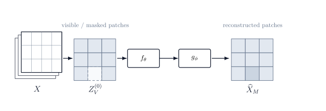
Breaking down the maths behind Masked Image Modeling

I have read and heard this thing multiple times: Masked Image Modeling.

I had a clue of what it was about, just by the name itself. You mask parts of an image and get a model to predict what has been hidden. Ok. But I am not satisfied with this. This is just a shallow understanding of it. In order to fully grasp something, I need to get my hands dirty and derive the maths. So that’s exactly what I am proposing to you in this blog post.

For us to understand Masked Image Modeling, we need to start from an image.

Let

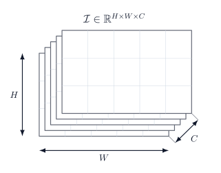
\mathcal{I} \in \mathbb{R}^{H \times W \times C}

where $H$ is the height of our image, $W$ is its width and $C$ the number of channels. A typical natural image would have three such channels (R, G, B). But when dealing with other types of images, like hyperspectral ones, you could easily have hundreds of them. Figure 1 is here to give you a sense of what this image can look like.

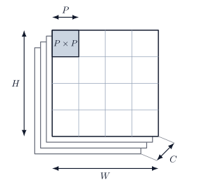
Figure 1: A stack of two-dimensional image planes with height, width, and channel dimensions.

In order to process such an image, it is usually common to divide it using non overlapping patches of size $P \times P$ such that the number of patches is:

N = \frac{H}{P} \cdot \frac{W}{P}.

You will sometimes hear people saying that they ‘patchify’ the image. Cute. Figure 2 can help you visualize what a patch is looking like.

A stack of image channels divided into non-overlapping P by P patches. — Figure 2: Dividing an image into non-overlapping patches.

Each patch can therefore be written as

x_i \in \mathbb{R}^{P^2 C}

Why is that? Because this patch is having an height of P, a width of P and a “depth” of C channels.

So now our image becomes

X = [x_1, \ldots, x_N]^\top.

Note that written as such, we have

X \in \mathbb{R}^{N \times P^2 C}.

In human words, this means that we now deal with an image, which is having N patches and each path is having $P^2 C$ elements.

From here we want to embed each patch. In order to do so we need to introduce a linear projection:

W_E \in \mathbb{R}^{P^2 C \times d}; \qquad b_E \in \mathbb{R}^{d}.

As you can see this linear projection is going to change the dimension we are working with (from $P^2 C$ we will move to $d$ ). Using this linear projection, our embedded patch is written as follows:

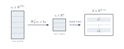
\underbrace{z_i}_{d \times 1} = \underbrace{W_E^\top}_{d \times P^2 C} \underbrace{x_i}_{P^2 C \times 1} + \underbrace{b_E}_{d \times 1} \in \mathbb{R}^{d}.

We can stack these embeddings such that

Z = \begin{bmatrix} z_1^\top\\ \vdots\\ z_N^\top \end{bmatrix} \in \mathbb{R}^{N \times d}.

and therefore we have with matrix notations:

Z = X W_E + \mathbf{1}_N b_E^\top \in \mathbb{R}^{N \times d}.

From Figure 3 you may get a sense of what we just did: we started from a patch with $P^2 C$ elements, we transformed it into one token of dimension $d$ , and we stacked those tokens together. In pratice however, all these operations happen with matrix multiplications just like you so with the previous equation.

A flattened image patch is linearly projected into an embedded token, and the tokens are stacked into the matrix Z. — Figure 3: Linear patch embedding turns each flattened patch into a token before the tokens are stacked.

Great. So now we have our tokens stacked together. Neat. What to do from here?

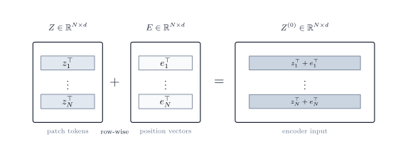
We are going to encode these tokens. In this following stage, we will be using self attention. However this mechanism does not have any notion of spatial position which is why we are going to introduce positional embeddings:

E = \begin{bmatrix} e_1^\top\\ \vdots\\ e_N^\top \end{bmatrix} \in \mathbb{R}^{N \times d}.

As you can see we have one positional embedding per token and if you look carefully $E$ does have the same dimension as $Z$ . That’s interesting, because it means we can sum them up.

So the actual input for the encoder will be

Z^{(0)} = \underbrace{X W_E + \mathbf{1}_N b_E^\top}_{Z} + E \in \mathbb{R}^{N \times d}.

Figure 4 is here to give you a visual clue of what we just did.

The patch-token matrix Z and positional-embedding matrix E are added row by row to form the encoder input Z superscript zero. — Figure 4: Positional embeddings are added row by row so each patch token carries its spatial position.

Now comes the time to mask patches. For this we need to define a masking ratio:

\rho \in [0,1].

We then sample a set of indices $M \subset \{1,\ldots,N\}$ such that

|M| = N_m \simeq \rho N.

Our set of visible indices is

V = \{1,\ldots,N\} \setminus M

such that

|V| = N_v = N - N_m.

We can rewrite our visible indices such that

V = (v_1, \ldots, v_{N_v}).

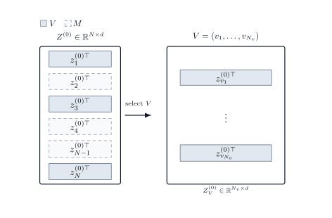
From here we retain only their corresponding embeddings:

Z_V^{(0)} = \begin{bmatrix} z_{v_1}^{(0)\top}\\ \vdots\\ z_{v_{N_v}}^{(0)\top} \end{bmatrix} \in \mathbb{R}^{N_v \times d}.

Figure 5 below shows one illustrative sampled mask. The dashed rows are masked, while the filled rows are the visible embeddings retained by the encoder.

An illustrative sampled mask keeps only the visible patch embeddings in the encoder input. — Figure 5: Sampling a mask selects visible rows from the row-wise token matrix $Z^{(0)}$ .

Now that we have the embeddings for our visible patches, it is time to encode them. We can define a vision transformer encoder like so:

f_\theta : \mathbb{R}^{N_v \times d} \longrightarrow \mathbb{R}^{N_v \times d}.

Now let

H_V = f_\theta\left(Z_V^{(0)}\right) = \begin{bmatrix} h_1^\top\\ \vdots\\ h_{N_v}^\top \end{bmatrix} \in \mathbb{R}^{N_v \times d}.

One way to understand this quantity is to say that each $h_j$ is a contextualized representation of the visible patch $v_j$ . This is due to self attention. Each token attends to the others to enrich its own context.

Now we are going to prepare the decoder input. Let’s assume the decoder works with a smaller dimension $d_D$ . Let’s project each encoder output using a new linear projection:

\underbrace{\widetilde{h}_j}_{1 \times d_D} = \underbrace{h_j}_{1 \times d} \underbrace{W_D}_{d \times d_D} + \underbrace{b_D}_{1 \times d_D}.

Let’s introduce a mask token

m \in \mathbb{R}^{d_D}.

Now we are going to reconstruct a sequence of length $N$ (the original number of patches).

For every original position $i$ , we have

\mu_i = \begin{cases} \widetilde{h}_j, & \text{if } i = v_j \in V,\\ m, & \text{if } i \in M. \end{cases}

This means that we are ending up with

Y \in \mathbb{R}^{N \times d_D}.

Here $Y$ , at position i, either holds a contextualized embedding of a visible patch which directly comes from our encoder, either holds a masked embedding for the patches we kept hidden.

Since the decoder needs positional embeddings, let’s define

E_D \in \mathbb{R}^{N \times d_D}.

Thus we have

Y^{(0)} = Y + E_D.

Figure 6 might give you a good overview of what we just did.

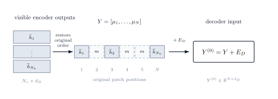
The decoder input is formed by restoring visible representations to their original positions, inserting the mask token, and adding positional embeddings. — Figure 6: Restoring visible representations and mask tokens to their original positions before adding decoder positional embeddings.

Now you may wonder why adding positional embedding here. Notice that for the masked positions, they are initially all having the same $m$ vector. Therefore adding its position indicates to the decoder which piece of the image it is supposed to reconstruct.

In order to decode, let’s define our decoder transformer as

g_\phi : \mathbb{R}^{N \times d_D} \longrightarrow \mathbb{R}^{N \times d_D}.

We have

D = g_\phi\left(Y^{(0)}\right) = \begin{bmatrix} d_1^\top\\ \vdots\\ d_N^\top \end{bmatrix} \in \mathbb{R}^{N \times d_D}.

We now have one representation $d_i$ for each original image patch.

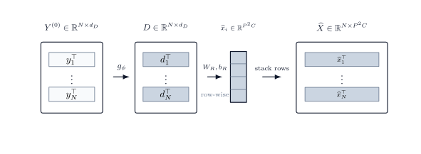
From here we want to go back to the pixel world. We need to remember that each patch contains $P^2 C$ pixel values. This means that we have to introduce the following linear projection:

W_R \in \mathbb{R}^{d_D \times P^2 C}; \qquad b_R \in \mathbb{R}^{P^2 C}.

Now for every patch we can write

\widehat{x}_i = d_i W_R + b_R \in \mathbb{R}^{P^2 C}.

We can stack these estimations such that

\widehat{X} = \begin{bmatrix} \widehat{x}_1^\top\\ \vdots\\ \widehat{x}_N^\top \end{bmatrix} \in \mathbb{R}^{N \times P^2 C}.

Figure 7 below summarizes the decoder and reconstruction path: each decoder representation is projected back into the pixel values of one patch, and the reconstructed patches are stacked into $\widehat{X}$ . Again, in practice, everything happens at the matrix multiplication level, we do not compute each element row wise and then stack, we just do matmul. I am voluntarily showing this here for educational purposes.

Decoder representations are projected row by row into reconstructed patches and stacked into the reconstructed patch matrix. — Figure 7: The decoder projects one representation per patch back into pixel space and stacks the reconstructed patches.

From here, we need a training objective. We are going to define one on the masked patches:

For this we can use a pixel-space mean square error (MSE):

\mathcal{L}(X,M) = \frac{1}{|M|} \sum_{i \in M} \frac{1}{P^2 C} \left\|x_i - \widehat{x}_i\right\|_2^2.

However please note that even though I am showing here this example of reconstruction happening in the pixel space, you could also consider reconstructing at the latent space. Figure 8 is here to convey a visual clue for our loss.

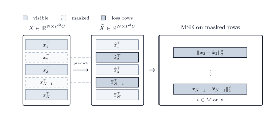
The original patch matrix X and reconstructed matrix X-hat are compared only on the rows corresponding to masked patches. — Figure 8: The model reconstructs every patch, but the training loss compares targets and predictions only at masked positions.

A few words here to understand the narrative. The model is allowed to see a number of visible patch. The encoder must therefore produce a useful representation of $X_V$ for the decoder to be able to estimate $p(X_M \mid X_V)$ . With the loss that we have defined, you can see that we are trying to minimize the difference between the real pixels (that we masked) and the estimations our model predicted for these.

In practice we usually set $\rho$ relatively high (e.g 0.75). Having a high masking ratio incentives the model to learn large scale structure rather than relying on local texture interpolation.

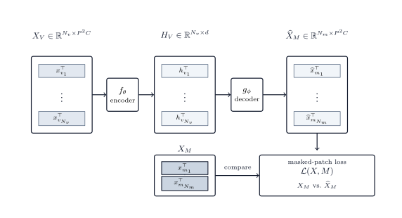
The complete training architecture looks like so:

X_V \xrightarrow{f_\theta} H_V \xrightarrow{g_\phi} \widehat{X}_M.

The masked image modeling training pipeline maps visible patches through the encoder and decoder to reconstructed masked patches, which are compared with the original masked targets. — Figure 9: Visible patches are encoded and decoded into masked-patch reconstructions, which are compared with the original masked targets.

Great! We made our way through Masked Image Modeling! Congrats!

From what I have understood, during pretraining the goal is mainly to learn the encoder $f_\theta$ and $g_\phi$ would be discarded. Later on $f_\theta$ can be used for classification, segmentation and so on.

I hope this blog post was useful. If you have any question, feedback or issues that need to be fixed in the post please feel free to reach out! :)