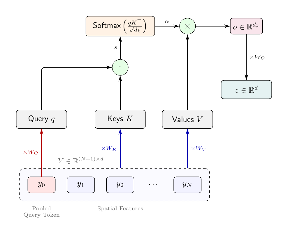
But what is attention pooling exactly?

Have you ever heard of attention pooling but never took the time to understand it? Well this is exactly what we are going to do in this blog post. Just sit down, and walk our way through the maths behind that concept.

The problem setting

Before anything, note that throughout, vectors are treated as row vectors.

Assume that you are working with a Convolutional Neural Network (a CNN). You are going to give it an image as an input and it is going to give you back a feature map.

You can define this feature map as:

X \in \mathbb{R}^{H \times W \times d}.

For the sake of illustration let’s assume $H = 7$ , $W = 7$ , and $d = 512$ . Here $H$ is the height of the feature map, $W$ its width, while $d$ is the dimension of each of the $7 \times 7$ vectors.

You can also rewrite this like so:

X = [x_1, x_2, \dots, x_{49}], \qquad x_i \in \mathbb{R}^{512}.

In this quantity, each $x_i$ is a feature vector for a given spatial location.

Great. So now what is the goal of pooling? Our objective here is to summarize this set of spatial feature vectors into a single fixed-sized representation. Mathematically, it looks like so.

We have a feature map:

X \in \mathbb{R}^{H \times W \times d}.

and we want to obtain $z \in \mathbb{R}^{d}$ , which captures the most useful information from the whole image. The different pooling methods you may come across simply differ in how they decide which spatial features should contribute to this summary.

Historic context

From what I have found, one early paper introduced the term of attentive pooling : https://arxiv.org/abs/1602.03609. In this paper they propose using learned attention weights as a pooling mechanism.

Later on, the OpenAI team while developing CLIP chose to adapt their ResNet architecture to use one layer of Transformer style multi-head QKV attention pooling. While doing so, they chose to use a query derived from the global average feature.

Average pooling

Now before understanding what attention pooling is about, let’s break down what a simpler kind of pooling looks like: average pooling. The formula for this is as follows:

z = \frac{1}{49} \sum_{i=1}^{49} x_i.

An equivalent way of writing it down is like so:

z = \sum_{i=1}^{49} \underbrace{\frac{1}{49}}_{\alpha_i} x_i.

We therefore understand that each location (each feature vector) gets the same weight $\alpha_i$ in the pooling (here $1/49$ ).

Attention pooling

Now, moving on to the attention pooling. This time rather than having the same weight for each feature vector, we are going to dynamically compute the coefficients from the image itself. In this section I am going to present attention pooling the way it is implemented in the CLIP paper.

Now let’s stick to our notation where:

X = [x_1, \ldots, x_N], \qquad x_i \in \mathbb{R}^{d}, \qquad N = HW.

So in our example earlier we had:

N = 7 \times 7 = 49, \qquad d = 512.

But from now on I will keep the abstract notations.

Pooling token and positional embedding

The first thing we are going to do is to compute a pooling token:

x_0 = \frac{1}{N} \sum_{i=1}^{N} x_i.

This is the exact same vector our earlier average pooling would have returned. Now let’s add this pooling token to our sequence:

\tilde{X} = [x_0, x_1, \ldots, x_N].

And we have:

\tilde{X} \in \mathbb{R}^{(N+1) \times d}.

Let’s define a positional embedding vector: $p_i \in \mathbb{R}^{d}$ .

We are going to add this vector to each vector from the sequence $\tilde{X}$ .

y_i = x_i + p_i, \qquad i = 0, \ldots, N.

And so we end up with:

Y = [y_0, y_1, \ldots, y_N] \in \mathbb{R}^{(N+1) \times d}.

Now we have a sequence of embeddings which are “aware” of the position. We have embedded the fact that $y_i$ encodes the $i$ th vector of the feature map.

Queries, keys and values

Starting from $Y$ , we are going to project it into queries, keys and values. For this matter, we need to introduce three learned matrices (one for the queries, one for the keys and a last one for the values). Let’s define them like so:

\begin{aligned} W_Q &\in \mathbb{R}^{d \times d_k}, \\ W_K &\in \mathbb{R}^{d \times d_k}, \\ W_V &\in \mathbb{R}^{d \times d_k}. \end{aligned}

Note that for clarity here I am going to omit the bias terms which are part of the linear layers.

In the way CLIP is implementing attention pooling, you do not need a query for every single token. Instead, the query comes from the pooled token we computed earlier:

q = y_0 W_Q.

Let’s compute the dimensions here. $y_0$ is a vector of dimension $d$ . As we saw just before, $W_Q$ has shape $d \times d_k$ . Hence, the resulting query $q$ has dimension $d_k$ .

Now that we have a query, we need keys and values. For these, every token provides a key and a value like so:

k_i = y_i W_K, \qquad v_i = y_i W_V, \qquad i = 0,\ldots,N.

where $k_i$ is of dimension $d_k$ and $v_i$ is of dimension $d_k$ . Notice that the pooled token $y_0$ is also going to produce a key and a value.

One way to conceptualize what is happening is that the average pool feature $x_0$ (later transformed into $y_0$ by adding a positional embedding) is asking the image which spatial features matter.

Attention weights

From here, we want to compute how relevant each spatial feature is to the global average pool query. Therefore, for each token, we compute:

s_i = \frac{q k_i^\top}{\sqrt{d_k}}.

Let’s break down the dimensions here: $k_i \in \mathbb{R}^{d_k}$ , so $q k_i^\top \in \mathbb{R}$ . That means $s_i$ is a scalar compatiility score.

Now we want to turn these scores into pooling weights. To do so, we are going to apply softmax:

\alpha_i = \frac{\exp(s_i)} {\sum_{j=0}^{N} \exp(s_j)}.

This does imply that

\alpha_i \ge 0, \qquad \sum_{i=0}^{N} \alpha_i = 1.

And this is now interesting to notice that while $\alpha_i = \frac{1}{N}$ , for the average pooling, we now have weights which are input dependent: $\alpha_i(Y)$ .

One important nuance to understand here though. While the matrices $W_Q$ , $W_K$ and $W_V$ are learned matrices, the attention weights $\alpha_i$ are not directly learned but they are rather dynamically computed from the image itself using learned matrices.

Ok, so now we have our attention weights. What to do from here?

Pooling

It is time to actually pool. We write down the output like so:

o = \sum_{i=0}^{N} \alpha_i v_i.

Now let’s stop for a minute here. We have computed our attention weights such that $\alpha_i \in \mathbb{R}$ . From the learned matrix $W_V$ earlier, we computed the values such that $v_i \in \mathbb{R}^{d_k}$ . So $\alpha_i$ is a scalar while $v_i$ is a vector. Hence, when we write $\alpha_i v_i \in \mathbb{R}^{d_k}$ , we are effectively scaling each vector by its importance, its attention weight. The resulting output is therefore $o$ such that $o \in \mathbb{R}^{d_k}$ .

Now if you go back to the section on average pooling, you may see that the final quantity we had was a vector $z$ resulting from this average. But so far we only have our output $o$ here, no $z$ yet. In order to get there we are going to apply a last learned linear projection:

z = o W_O.

The dimension of $W_O$ is:

W_O \in \mathbb{R}^{d_k \times d_{\mathrm{out}}}.

In the average pooling example from ealier we had $z \in \mathbb{R}^{d}$ , so here for simplicity let’s assume $d_{\mathrm{out}} = d$ .

If you made it so far, then congrats because you just learned what is attention pooling for a single head! The toughest part is done. But I can’t let you go without mentioning multi-head attention pooling.

Going multi-head

Now, suppose we have $h$ heads. For each head $r$ with $r \in \{1, \ldots, h\}$ , we are going to give it its own projections: $W_Q^{(r)}$ , $W_K^{(r)}$ , and $W_V^{(r)}$ .

Then each head is going to independently repeat what we just learned before:

\begin{aligned} q^{(r)} &= y_0 W_Q^{(r)}, \\ k_i^{(r)} &= y_i W_K^{(r)}, \\ v_i^{(r)} &= y_i W_V^{(r)}. \end{aligned}

Then:

s_i^{(r)} = \frac{q^{(r)}\left(k_i^{(r)}\right)^\top}{\sqrt{d_h}}.

Then:

\alpha_i^{(r)} = \frac{\exp(s_i^{(r)})} {\sum_{j=0}^{N} \exp(s_j^{(r)})}.

And finally:

o^{(r)} = \sum_{i=0}^{N} \alpha_i^{(r)} v_i^{(r)}.

Now, if each head has dimension $d_h$ , we have:

o^{(r)} \in \mathbb{R}^{d_h}.

From here, we concatenate them:

o_{\mathrm{cat}} = \left[o^{(1)}; \ldots; o^{(h)}\right] \in \mathbb{R}^{h d_h}.

We usually choose $d_h$ such that $h d_h = d$ . That means:

o_{\mathrm{cat}} \in \mathbb{R}^{d}.

Then we have our usual final projection:

z = o_{\mathrm{cat}} W_O, \qquad W_O \in \mathbb{R}^{d \times d_{\mathrm{out}}},

and remember that we can take $d_{\mathrm{out}} = d$ .

The way to conceptualize this is simply to understand that we perform several independent attention pooling operations whose outputs are concatenated and linearly mixed.

Closing thoughts

The toughest part of understanding attention pooling comes from understanding the attention mechanism itself and keeping track of the different dimensions we are dealing with. I thought it could be nice to write down the maths behind in order to really understand what is going on and I would suggest you to do the same whenever trying to understand something: going back to a pen and a paper and write down the math!