Motivation
On November 6th, Meta unveiled e-means, claiming to outperform K-means in one-tenth the epochs: https://arxiv.org/abs/2611.09501
It got me curious and I felt like before reading their paper, I would jump back to reading about K-means again in order to fully understand their contribution. I didn’t really know what would be the best resource to revise this algorithm. But eventually while skimming through potential candidates, I have settled with watching this lecture on Youtube: https://youtu.be/LmpkKwsyQj4?si=5Fl5QCadtty5z-qB
It is a lecture from Dr. Anand Avati at Stanford (CS229). All the following will be based on his lecture and the notes I took while watching it.
On a personal note, I think we are extremely gifted to have such amazing content online for free, from the best universities in the world, just waiting out there for anyone to learn from!
So in the following part of this post, my goal is simply to put my notes into words regarding this algorithm and how it is presented in this lecture. I think it is a very good way for you to have a quick reminder on this algorithm and a great way for me to revise it again :)
Supervision or not?
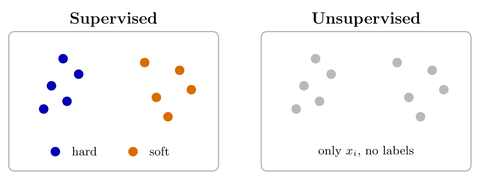
Suppose we have a dataset of cheese images. After passing these through an encoder you would end up with one embedding for each of your images. This would results in the dataset . In a supervised setting we would have a set of associated with those . If you would like to formalize it, it could be . If your goal is to know whether your cheeses are hard or soft, this supervision could be .
However for K-means, we are working in an unsupervised setting, which means that in our case we only have and our goal is to figure out some interesting structure in our data in the absence of supervision (i.e in the absence of ). Figure 1 showcases the difference between the two settings.
When you think about it, an unsupervised setting is the case you are going to encounter the most when dealing with data. You are likely to stumble upon messy pieces of text or a random image. You are less likely to find a clean labeled dataset for your task.
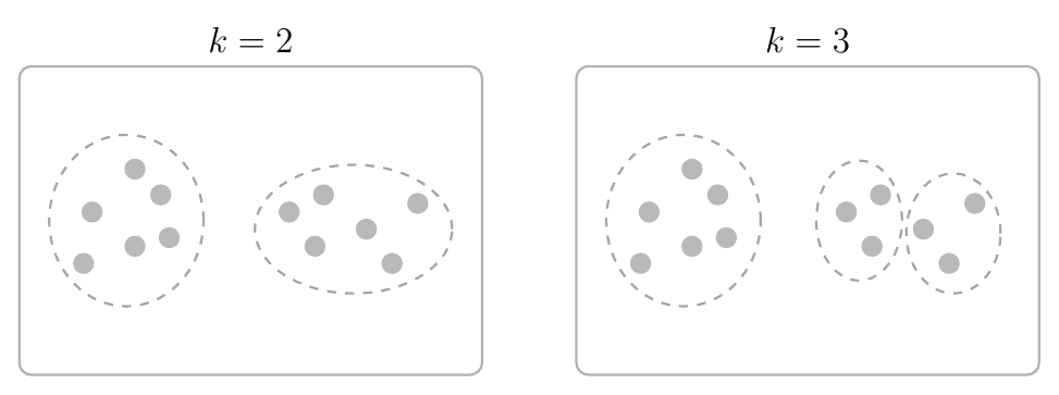
Now as you can see in Figure 1, in the supervised setting there is usually some ground truth hyperplane that cleanly separates hard cheeses from soft ones. However in the unsupervised setting, the correct answer can be more blurry. As illustrated in Figure 2, you might encounter situations for which it is equally reasonable to find two or three clusters. The “correct” answer is less obvious.
The K-means algorithm
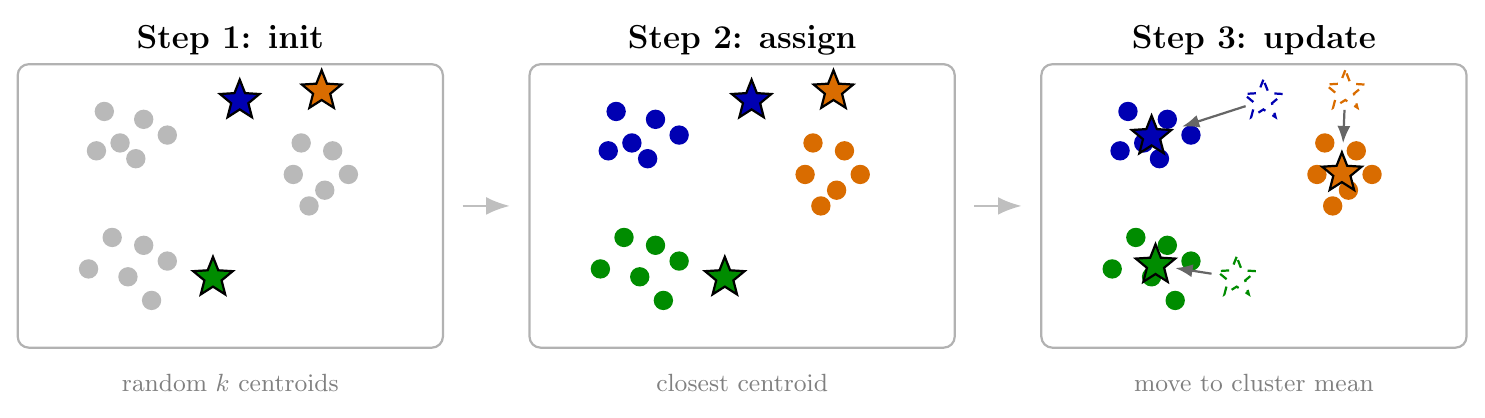
Now how do you actually cluster your cheese images? Well that’s when K-means comes in. It is a pretty straight forward algorithm which goes like this.
First you are going to define your dataset where . You also need to define as the number of clusters you want your algorithm to find. Given this you need to follow these steps:
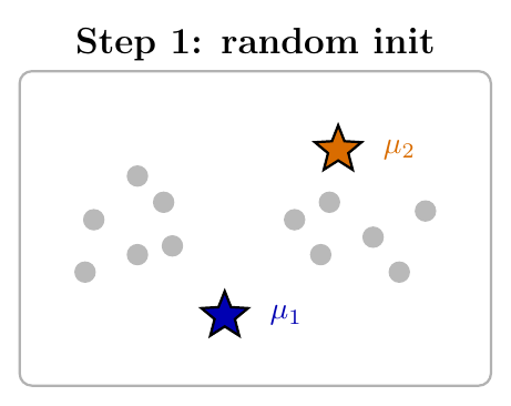
- You randomly initialize cluster centroids which we are going to name here. Each also belongs to . This initialization is being shown in Figure 3.
- Then you are going to repeat until convergence the following (do not freak out, we are going to break down the math):
(*) For every , set
(**) For every , set
Ok, we need to break down what is happening here.
Let’s start with (*).
Here is the formula:
For every , set
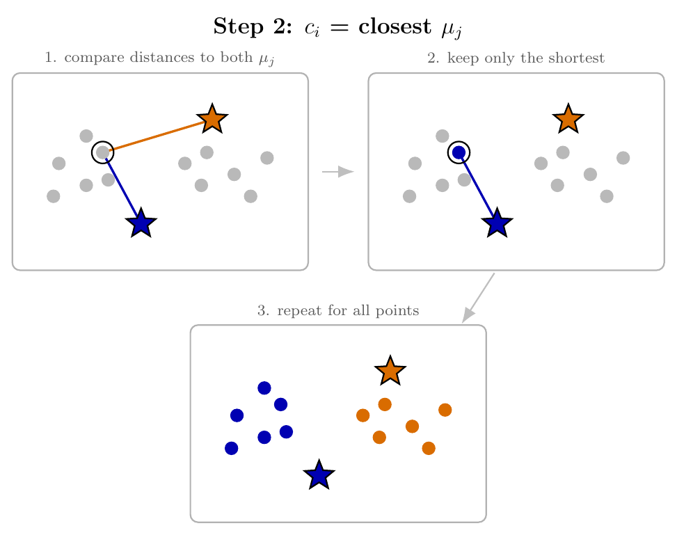
In other words, for every (every cheese image embedding), we are going to define a . Now, that is the identity of the closest cluster centroid. As shown in Figure 4, for a given data point (here the circled blue dot), we are going to check which cluster is the closest. In the case of Figure 4, that’s the blue star. And you need to do that for each data point. So now you have and , each being the closest cluster identity to . As written takes its values in because of the argmin.
Now we need to understand (**) which says:
For every , set
That one is maybe a little trickier to grasp. The first thing to understand is the indicator function. The indicator function takes a condition and returns if it is true and if it is false:
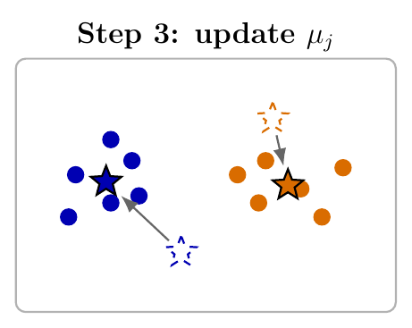
Ok. Now that we are ok with that let’s look at our formula. What is happening here is that we are going to recompute the cluster centroids. Each cluster centroid is going to be recomputed as the mean of all its data points, and what I mean by “its” here is: all the data points for which is the closest cluster centroid.
So in other words, for the cluster centroid , if the indicator function returns 1, it means is the closest cluster centroid for the data point and therefore we want to include in our sum, otherwise we don’t: .
Now you do that for all data point and divide by the number of data point in your mean and you get the new value for your cluster centroid. An illustration of this process is given in Figure 5.
In practice it can be shown that K-means always converges to a local minimum. The loss function this algorithm minimizes is named the Distortion Function and is written as follows:
What this function says is that we are trying to find a set of and such that the squared distance between all data points and their assigned cluster centroids is as small as possible.
As you saw earlier, this algorithm is alternating between two different steps. In one step it optimzes with respect to and in another it optimizes with respect to . We say that K-means is coordinate descent of the Distortion Function.
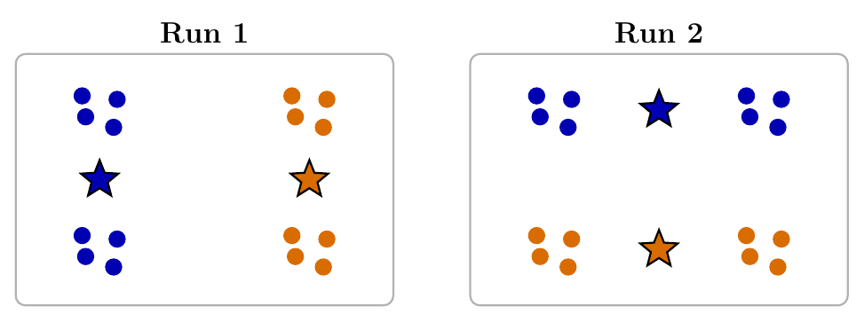
Lastly, since it can be shown that is a non convex function, we may end up with a different set of and depending on the initialization chosen (Figure 6).
And here you go! That’s what there is to know about K-means, now it’s time to read the paper from Meta on e-means :)
Acknowledgements
Many thanks to my friend Aritra for giving me valuable feedback on this post.